Skipper NDT x HETIC — Intelligent Pipeline Identification by ML
A 3-week industrial ML project in partnership with Skipper NDT, a world leader in non-destructive testing of buried infrastructure. The mission: develop machine learning models to automatically analyze multichannel magnetic field maps and extract key parameters from underground pipeline data — replacing manual expert analysis.
4
ML tasks (classification + regression)
2 833
NPZ magnetic images analyzed
1.000
Recall T1 — zero pipeline missed
1.47m
Best MAE — T2 magnetic width
Industrial Context
Skipper NDT uses drone-mounted magnetic sensors to detect buried networks (oil, gas, water, electrical cables) without excavation. The active magnetic field detection generates high volumes of 3D data that experts must manually interpret — a slow, error-prone process. The goal: automate analysis with ML so that field agents without signal expertise can make decisions autonomously.
Data format
Multichannel TIF/NPZ images — 4 channels: Bx, By, Bz, Norm (nanoTesla). 1 pixel = 0.2m. Highly variable dimensions: 150×150 to 4000×3750. ~86% NaN values (unmeasured zones outside acquisition corridor).
Key challenge
NaN values are not just noise — they carry geometric information about the acquisition zone. Resizing destroys the absolute physical scale (1px = 0.2m), making standard image regression approaches invalid for metric prediction.
The 4 Tasks
Pipeline Presence Detection
Binary classifier: does the magnetic map contain a pipeline? 2,833 NPZ images (1,700 positive / 1,133 negative). The key methodological decision was adding an explicit NaN mask as a 5th channel — preventing the model from confusing a true zero magnetic response with an unmeasured zone.
Architecture
SmallCNN (5 channels) + BCEWithLogitsLoss + AdamW
Accuracy / Recall
0.997 / 1.000
Target
Accuracy >92% · Recall >95% — both exceeded
Magnetic Map Width Estimation (Regression)
Predict the effective width of the magnetic influence zone in meters. The fundamental constraint: 1 pixel = 0.2m is an absolute physical relationship. Any global resize destroys this bijection, invalidating metric regression. This forced a complete paradigm shift toward direct geometric measurement.
Methods explored — from failed approaches to winning solution
| Method | MAE | R² | Status |
|---|---|---|---|
| EfficientNet-B0 — resize 224×224 | 8.1m | 0.87 | Resize destroys scale |
| EfficientNet-B0 — padding 512×512 | 9.6m | 0.82 | CNN without absolute scale |
| TCN — 1D interpolated profiles | 18.3m | 0.45 | Interpolation deforms width |
| XGBoost + NaN scan (FWHM) | 4.9m | 0.93 | Arbitrary threshold |
| XGBoost + multi-sigma spatial gradient | 3.68m | 0.97 | Best XGBoost approach |
| PCA + Rotation + Patch + MAX non-NaN pixels | 1.47m | 0.98 | Best method — native resolution |
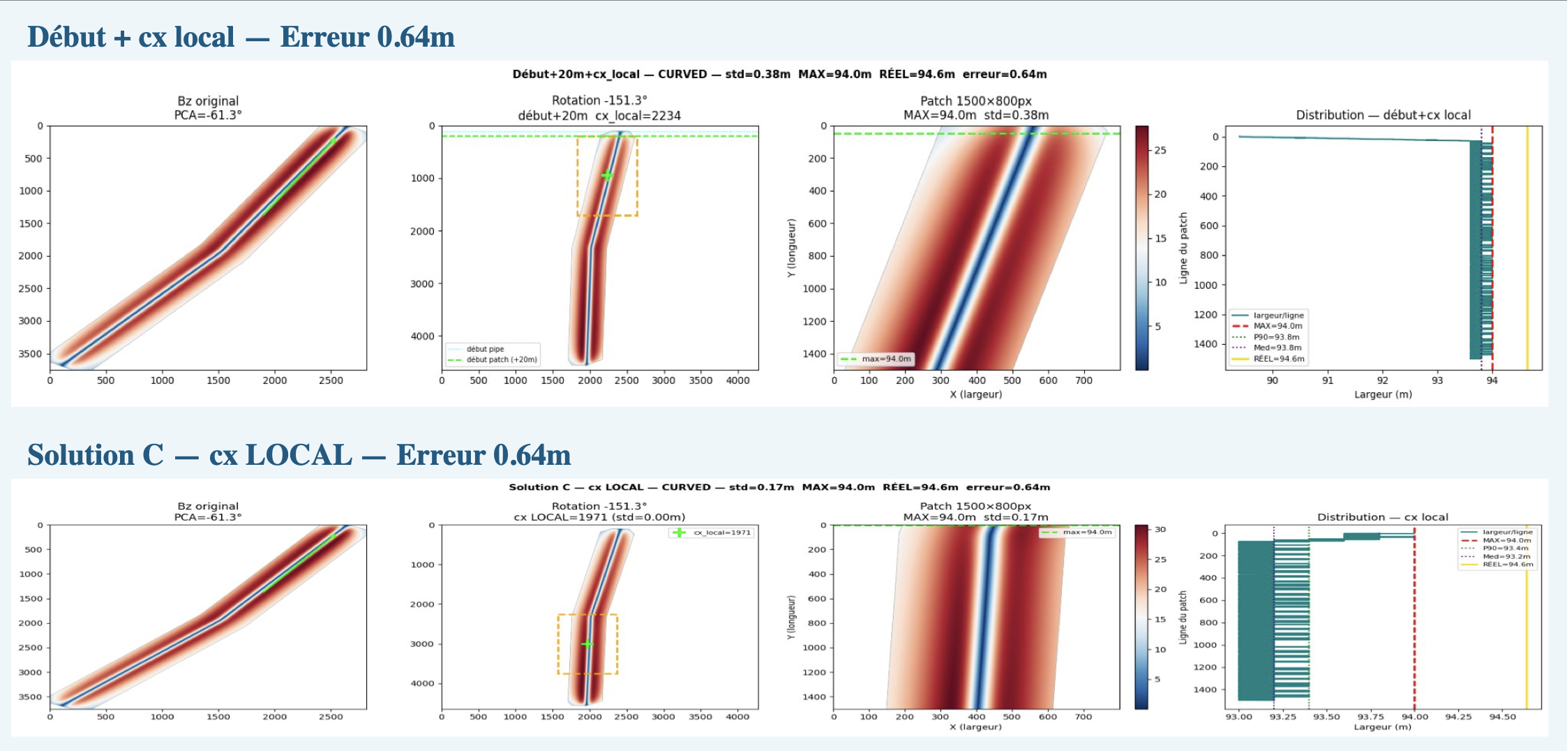
Final winning method — 4 steps
PCA on the top 5% strongest pixels of the Bz channel to estimate the pipeline orientation angle
Rotate to make the pipe vertical. NaN zones rotated separately via a binary mask — preserving their physical meaning
Extract patch at pipe start +20m offset, with adaptive width if signal saturates
Count non-NaN pixels per row in the patch → convert to meters via 0.2m/pixel. No model predicts the width: it is measured geometrically.
MAE straight pipes
0.334m
MAE curved pipes
6.836m
R² (measured cases)
0.9813
Coverage
482/1700
Limit: global PCA rotation fails on curved pipes. Next iteration: local segment detection + adaptive patch height to cover 100% of the dataset.
Current Intensity Classification
Binary classifier: is the injected current intensity sufficient for reliable magnetic detection? 4,715 samples (2,829 detectable / 1,886 non-detectable). Key insight: unlike Task 2, resizing is acceptable here because the target is classificatory — the model recognizes a signal pattern, not a metric quantity.
Architecture
EfficientNet-B0 (4 channels) — ACP rotation + resize 224×224 + 2-phase fine-tuning
Accuracy / F1
92.37% / 0.9365
Recall (class 0)
93.65%
Parallel Pipelines Detection
Binary classifier distinguishing single pipeline images from parallel pipeline configurations. Harder problem: detecting subtle spatial repetition and parallelism patterns. ~300 samples — smaller dataset raising overfitting risk.
Architecture
CNN embedding extractor + XGBoost classifier — hybrid approach
Internal accuracy
~99%
Note
External validation required to confirm generalization
Key Scientific Learnings
NaN is not noise — it is physical information
Adding an explicit NaN validity mask as an extra channel was a decisive modeling decision, not an implementation detail. It prevents the model from confusing unmeasured zones with true zero magnetic responses — directly impacting T1 and T4 quality.
Resize does not have the same meaning depending on the target
For pattern classification (T1, T3, T4): spatial normalization is acceptable, even necessary. For an absolute metric target like width_m (T2): it becomes destructive. This distinction forced us to break from standard image regression and invent a geometry-first approach.
Hybrid approaches outperform pure deep learning when geometry is explicit
CNN + XGBoost (T4) and PCA + geometric measurement (T2) both outperformed end-to-end deep learning. The best strategy uses neural networks to extract complex visual representations and leaves rule-based or tabular models to make final decisions — especially when physical constraints are knowable.